Quantum Fractals - The Algorithm |
|||
 |
|||
|
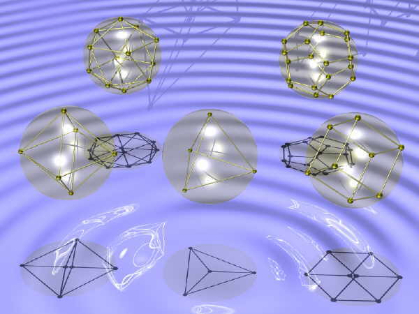
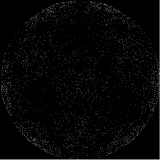
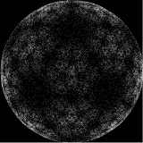
In applications the vectors n[i], i=1,2,...,N can be arbitrary except that they are of unit length, that is they all lie on the surface of the sphere of unit radius, and they add to zero vector: n[1] + n[2] +...+ n[N] = 0 - so they are balance each other in such a way that their common center of gravity is at the center of the sphere. The algorithm describes a sequence of maps of the sphere. These maps are applied, sequentially, to a randomly chosen starting point. Thus what we get is a point on the sphere jumping in a somewhat chaotic way on the surface of the sphere. After 100 000 jumps or so a pattern appear. This pattern is independent of the starting point, as it is usual in chaotic dynamics with an attractor. What we see is an approximation of the attractor set. For instance, for a particular value of the fuzziness parameter alpha = 0.65, and the dodecahedron, we get the following images for 10 000,100 000, 1000 000 and 10 000 000 respectively: |
|||
 |
 |
 |
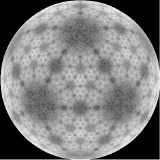 |
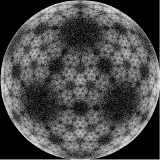
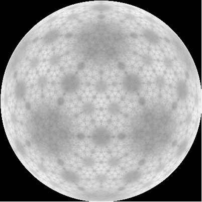
| The more jumps we generate, the more details of the attractor set shows up. The 100 000 000 dots image shows even more details: | |||
|
Given a point r the algorithm first computes probabilities p(i,r) of sum 1: p(1,r)+p(2,r)+...+p(N,r) = 1 with which we select the map that is to be applied to r. The formula, explained in more details in the paper, reads: p(i,r) = (1 + alpha2 + 2 alpha n[i].r )/( N( 1 + alpha2 )) where n[i].r stands fro the scalar product of n[i] and r, that is, in our case, for the cosine of the angle between the vectors n[i] and r, and alpha is the "fuzzy" parameter 0 < a < 1 . Once, for a given current point r, the probability distribution p(i) = p(i,r) is computed, a vertex n[i] is selected accordingly. Here we follow the standard procedure of selecting a case according to the given probability distribution. In Java code: |
|||
|
|||
|
Then the new point r' on the sphere is generated using the following transformation: r ' = ( (1 - alpha2)r + 2 alpha( 1+ alpha n[i].r )n[i] )/( (1 + alpha2 + 2 alpha n[i].r ) ) |
|||
| The denominator here is nothing but the length of the vector in the numerator, so as to ensure that the resulting vector is of unit length again. This normalization is the only nonlinearity in the resulting "iterated function system" (IFS). | |||
|
Rendering of the image Once the data are collected in a pixel array d[i,j], they need to be converted into a picture, either using grayscale or some coloring scheme. For instance one can find the maximum m = max (d[i,j]) divide it into 256 equal intervals, and aasign a grayscale value between 0 and 1 to an (i,j) pixel according to the value of d[i,j]/m. In fractal images it is neccessary to make some transformation of the array values before, otherwise details of the pattern are lost. For rendering of the greyscale pictures above we have used log10(log10(d[i,j]+1)+1) transformation. |
|||
Under construction:EEQT OpenSource ProjectImage gallery ...Prticle tracks, Tunneling times ...Beta wersion of Win9x application Note: These two applets crash on certain browsers. Internet Explorer seems to be OK and Mozilla seems to be OK. The applets crash with Opera (for reasons that are not understood) and with older Netscape. Therefore the best thing is to download the .jar files from SourceForge, unpack them, download Java SDK appropriate to the operating system, install it, and then run the .jar files with "java -jar qf.jar" or "java -jar wave.jar". |
|||
|
|
|||
 There
are two separate problems when creating these fractal images, namely
that of generating data, and of rendering the generated date into an
image.
There
are two separate problems when creating these fractal images, namely
that of generating data, and of rendering the generated date into an
image.